|
|
|
|
|
|
A Mapping is composed of components. Each component defines part of the processing to be performed by the Mapping. All components are optional, except that each Mapping must contain a level-type component called Main.
The relationships between the components of a Mapping can be illustrated with a simple, generalised diagram:
Diagram qed040
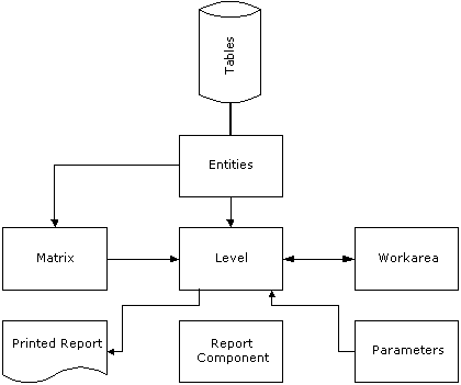
Parameters are used to specify what data is to be extracted and processed by the Mapping. Data is extracted from tables via entities; it may be processed directly by the level component, or be summarised in a matrix; the workarea component defines temporary storage used by the Level for intermediate results. The level finally uses line definitions set up in the report component to format the processed data and produce a printed report. This simplified description shows that level components are at the heart of all Mappings.
A Mapping can have any number of level components, but the level called Main (which must exist) is always the first component invoked when the Mapping is run.
The parameters component defines data required by the Mapping when it begins to run. This may be entered by the user, or it may be obtained from another program via a commarea. (Parameters may be defined individually within the Mapping, or else the Mapping can make use of a pre-defined parameter group.)
The matrix component defines the data to be collected from the database and the way it is to be structured and summarised before it is processed by the levels.
The workarea component defines temporary variable storage to be used by the Mapping as it runs; this can include individual intermediate calculation results and simple counters and even large arrays of similar values.
The report component defines the output from the Mapping - the way the results of the processing are presented to the user. This includes the layout of the report, with page headers and footers and the way individual items of data are displayed in fields.
The level components define the processing to be performed by the Mapping. This includes all the calculations (such as subtotalling) and the instructions to print particular lines of the report (as defined in the Reports component). The data processed usually comes from a database; this is selected and extracted according to specifications in the parameters and matrix components. The processing definition is given in terms of MDL, the Mapping Definition Language at the core of QED itself. MDL provides you with a set of commands and functions which are used to give step-by-step instructions to QED on how to manipulate data.
It is important to understand the relationship between levels and reports.
Reports are normally laid out in sections, with subtotals at the end of each section. The subtotals for all the sections are combined into a grand total at the end of the report. The sections themselves may be subdivided and the subdivisions have their own subtotals which are incorporated into the section subtotals; and so on.
QED allows the use of two methods of handling this kind of structure.
The first method uses a separate level component to handle the processing and subtotalling for each section of the report. (Subtotals occur at total breaks. These are also often referred to as control breaks.) This is called nesting: one level component calls another to perform a particular piece of processing, which may be repeated many times and the called level may itself call another. (There are no practical limits to depth to which levels may be nested.)
The second method uses level breaks (corresponding to control breaks) within a single level component.
Consider, for example, a report which lists products sold. These are to be grouped into product types, sales region and period. This means that the detail lines in the report will be sorted into product types within regions within periods. Subtotals will be produced when the product type changes, when the region changes and when the period changes.
The structure of the report and therefore of the associated processing, is represented by the diagram:
Diagram qed050
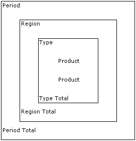
The nesting of the boxes corresponds to the different levels of processing. Processing in the innermost box (Level 3) is repeated most often and the outermost box (Level 1) is repeated least often.
All the products of the same type are listed and a total printed, at the lowest level of processing (Level 3). This is repeated for each product type, until all the products sold within a region have been printed and a total for the region is printed at the next higher level (Level 2).
Next, the products sold in another region are listed, totalled by product type; a total for this region is printed. When all regions have been totalled and printed, a total for the period is printed and the next period is processed (Level 1). When all periods have been printed, a total for the report is printed and processing stops (this can be regarded as Level Zero).
The instructions to print product information (product name, quantity sold, value of sales) are contained in Level 3; these are executed for every product line. The instructions for printing region information (region name, total number of products sold, total value of products sold) in Level 2 are only executed when all of the product types sold within the region have been processed. This level is executed once per region. The period information is printed once per period, after all regions have been processed. When all periods have been processed, a grand total is printed.
First, consider how this would be handled using a separate level component for each level of processing and reporting.
The Main level (Level Zero in our example - not shown in the diagram) starts everything off: it prints the report title, clears a set of variables which will be used to accumulate subtotals, then performs Level 1. (When one level performs another, its processing is suspended and the invoked level runs. When the invoked level stops, the performing level re-starts where it left off. This is known as passing control from one level to another.)
Level 1 prints the subtitle for the first period, clears an independent set of variables for accumulating subtotals and performs Level 2.
Level 2 prints the subtitle for the first region, clears its own set of accumulators and performs Level 3.
Level 3 prints the subtitle for the first product type, clears another set of accumulators and prints a detail line for each product of the current type, adding the values to the subtotal variables as it goes. When it has printed the last line for the first product type, it prints a subtotal line, then stops and control returns to Level 2.
Level 2 adds the Level 3 subtotal values to the Level 2 accumulators. It prints the subtitle for the next product type and performs Level 3 again.
Level 3 prints the product type subtitle, clears its accumulator variables, then prints the detail lines, accumulating the new values for its subtotals, until all products of the current type have been printed. It prints a subtotal line and returns control to Level 2. Level 2 adds the Level 3 subtotals to its own accumulators, prints the subtitle for the next product type and calls Level 3 again.
When Level 3 has printed the last subtotal for the last product type, it returns control to Level 2. Level 2 prints the subtotal for the region and passes control back up to Level 1, which accumulates the Level 2 subtotals. It then passes control back to Level 2 for the next region to be processed.
So the processing continues, with control passing up and down between levels until all the data has been listed and the subtotals at each level have been printed. Eventually, control returns to the top level, Main, which prints the grand totals and then stops.
It is worth taking time to follow through this example and make sure that you understand the principles involved, because it will make the job of designing Mappings and reports much easier. (The preceding description contains some simplifications, such as omitting a description of how to print section headings at the top of each new page, but these are not important to an understanding of the principles being discussed.)
Now, exactly the same thing can be achieved within a single level component.
Within any level component, there are several blocks available for entering MDL instructions. Each block is executed at a different stage in the execution of the level. The first and last blocks, known as Pre-Process and Post-Process respectively, are only executed once each time the level is executed, but they are always executed, whether there is any data to process or not. The pre-process block is usually used to print a heading (such as column labels) and the post-process block usually prints total or subtotal lines. If there is only one level component Main, then pre-process and post-process will print the report title and trailer pages.
The process block, in the middle, is the one which is executed when there is data to process. It is executed once for each instance of the entity which the level is processing. (If there are other level components in the Mapping, then they are usually executed by PERFORM commands contained in the process block.)
So far, this is true of all levels. Now the new method of using Level Breaks allows the introduction of more blocks of MDL between the pre-defined blocks just described. This means that instead of having a PERFORM statement which calls another level to perform processing based on a different entity, you can just Insert another Break in the current level.
One major advantage of doing things this way is that you can see and understand the structure of a Mapping at a glance on one screen. It is easier to move from one block of MDL to another and you don't have to remember which level calls which and in what order.
(See Levels Overview and 'MQM0 Level Break - Amend' for details of how to set up breaks within a level.)
The two methods are conceptually the same, but level breaks are somewhat more efficient as well as being easier to use. The older method (with a separate level component for each control break) has always been available in QED; level breaks were introduced with version 4.4 specifically to cope with particular situations which were difficult to handle using separate level components. Either style of level usage may be used according to preference in the majority of cases.
When a Mapping created with an earlier version of QED is amended and saved using the current version, then it is automatically converted to the new style. (Old Mappings developed and compiled with earlier versions will of course continue to work as before.)
Workareas contain workfields. A workfield is a unit of temporary storage used to hold intermediate or calculated values whilst a Mapping is running. A workfield can hold data of the class which is assigned to it when it is defined. (A workfield definition is sometimes called a declaration.) Most workfields hold single values, but a workfield can be defined as an array, which can hold many values. All the values stored in an array must be of the same class. Because the contents of a workfield can change, it is often called a variable.
Workfields defined in a workarea are global - that is, they are available to all components of the Mapping. This contrasts with workfields defined within levels, which are local to the level in which they are defined.
Parameters are like workfields, in as much as they are variables used to hold values which a Mapping needs whilst running. They differ, however, in that they receive their values from outside the Mapping - either entered by the user when the Mapping is run, or obtained from another source (often another Mapping or program) via an area of storage known as a Commarea. For example, a Mapping which produces a report summarising information across a period is given the start and end dates of the period when it is executed.
Parameters can be defined individually for each Mapping, or else a pre-defined parameter group can be used. Many Mappings require similar sets of run time data; a parameter group includes full definitions of such regularly required parameters, providing validation and default values. Mappings which make use of standard parameter groups can be developed more quickly, especially if large numbers of parameters are required.
Although workfields' values will change many times, parameters normally retain the same value whilst a Mapping is executed (for example, the start and end dates mentioned above will usually be printed in the header at the top of each page of the report). Their values are assigned to them when the Mapping starts to run.
Almost all Mappings extract their data from the database via one or more entities. An entity is a model of a real-world object that you want to process. For example, products, invoices and assets are things in the real world which are represented within QED by entities. Entities have attributes; attributes are things that are known about the entity. For example, an invoice will have attributes such as invoice number, date issued, net value and so on; a product will have attributes such as stock number, name, size, colour, weight and so on.
Entities conceal the structure of the underlying database and make it easier for you to use the data held in your system. The data in your system is stored in a way that maximises efficiency and security and reduces storage requirements; this can mean that items of data which you regard as being similar or related may actually be kept in apparently unrelated places in the database. As an example, consider an entity called Product; one of its attributes is likely to be Current_total_stock. It is actually quite unlikely that a single number representing the current total stock of an item is stored anywhere in your database; what you will normally have is a group of numbers representing the amounts of stock in several different locations. The function of the attribute Current_total_stock is to consolidate those several quantities into a single number, the total amount of stock on hand. The entity Product converts the data in the database into information which you can use.
A matrix is quite a complex construction, so inevitably takes some time to set up. The design of a matrix should be developed on paper before sitting down to build one into a Mapping.
You should understand what a matrix is and how to use one to solve problems in creating complicated reporting structures.
A Mapping can contain any number of matrix components (the plural of 'matrix' is 'matrices'). Each matrix must have an entity or table associated with it.
Table Devices provide a similar service to entities, in that they are used to hide the structure of one thing, to make it look like another. Their main use is to make external data sources look as though they are part of the database. For example, you may have a sequential file containing details of transactions that you want to process. The Mappings that you develop can normally only work with entities based on tables in the database; you can define a table device to make the sequential file look like a table and make it accessible to your Mapping.
There can only be one table device component in a Mapping.
See also
QED Mapping Development Home Page
|
© Advanced, Jan 2021 |
|